Introduction

When you turn on a household tap, have you ever wondered how the water gets there? There is a maze of underground pipes ensuring you have a reliable supply of water. Selecting the size of these pipes is an extremely difficult undertaking: they are not cheap, and we would like all customers to get a similar quality of water supply.

About the game

The Aqualibrium competition was established by a South African academic, Kobus van Zyl, and has been played by students from all over the world. The task is to connect 3 reservoirs through a network of pipes and ensure they get an equal supply of water. However, there are some decisions to make. You can use up to 12 large pipes (6mm), and up to 12 small pipes (3mm), or for up to 8 locations you can choose to not have any pipe. This leads to many millions (see below) of possible combinations of networks you might design. Additional rules are that you may not have dead-end connections and you can only have a maximum of 4 pipes at a junction, including the reservoirs

Detailed explanation of the rules can be found here

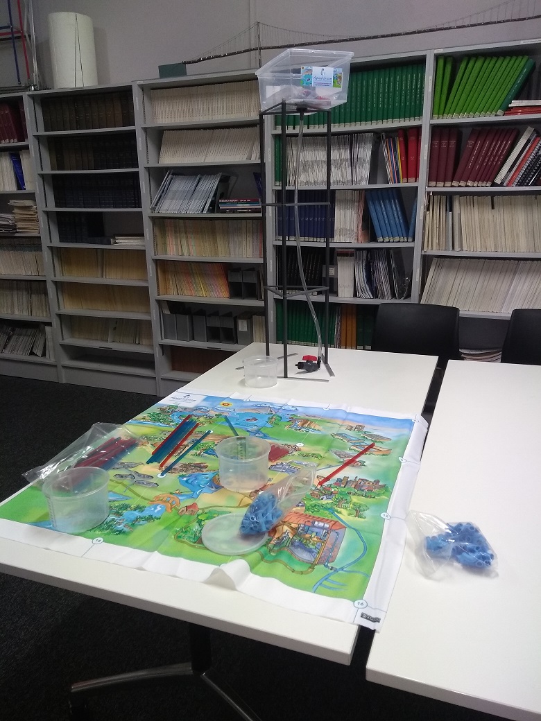
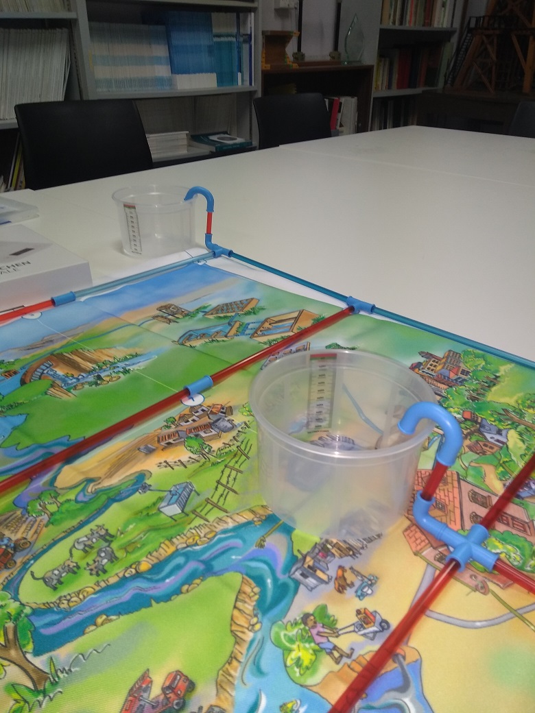
Some example pictures of the physical equipment: Network materials Network connectors

About this site

Ths website has been established so you can analyse the network and find good designs. Click on the mid-point of a pipe to cycle through the 3mm diameter (blue pipes), 6mm diameter (red pipes) and no-pipe options for that link. The flow in each pipe is solved in the background using a program called EPAnet, which is a program taught in universities and used by civil engineers for analysing water networks. Conceptually, the model determines the 'path of least resistance' based on the friction of the pipes (bigger pipes have less friction effect). Some checks have been implemented to make sure your network is valid according to the competition rules. Flow is measured in litres per second L/s. Pressure values can be displayed using the Options menu, and are measured in units of metres (these units can be interpreted that if a hole were in the top of the pipe, a jet of water would jump to that height).

Are my results correct?

This is a very important question and the subject of entire university courses in water engineering. The model on this website is simplified when compared to the real physical network used in the competition. The model makes a number of assumptions and simplifications - some of which are not important, but some of which might lead to a very different set of results. For example, the model is not a time-varying analysis, it calculates flows and pressures once-off based on the initial water level. You will not find a long list of simplifications/assumptions here, because we want you to think about what might not be taken into account in the online model. One hint is that there are additional locations of resistance that are not properly accounted for in the model, where the water burns off energy due to extra friction or turbulence.

How many combinations are there?

There are 24 pipes. Assuming only 2 diameter options (3mm and 6mm) at all locations gives a lower estimate 2^24 = 16 million options. Assuming 3 diameter options (3mm, 6mm, no-pipe) at all locations gives an upper estimate 3^24 = ~282 billion options. But the true picture is more complicated.

There are upto 8 pipe locations with a 'no pipe' option. Combinations of locations of 8 missing pipes from 24 locations is 735,471, with 2^16 options for the pipe diameters. Repeating this calculation to allow for cases only having 7, 6, ..., 1, 0 missing pipes gives a more accurate estimate of ~167 billion cases. However, this is still an overestimate because the condition that there are only 12 pipes maximum for a given diameter (whether 3mm or 6mm) is not accounted for... which you might be able to work out by removing from the 2^16 options the number of cases with more than 12 pipes of one type. Even doing this, is still an over-estimate because we haven't thrown out the dead-end cases.. but that is a very hard condition to account for as we would need to consider the connectivity of the network...regardless, the number of options is likely to remain in the billions. Lastly, note that this is a small network, real world networks have many more pipes.

Program Info

The web interface was written using RShiny 1.0.5 and R 3.4.3. I am especially grateful for the epanet2toolkit package in R by Brad Eck which provides key functionality for accessing the EPAnet network solver from the R environment.